Fitting autocorrelograms
In the processing pipeline, the autocorrelograms of each cell is parametrized using a triple exponential equation:
ACG_fit = 'max(c*(exp(-(x-f)/a)-d*exp(-(x-f)/b))+h*exp(-(x-f)/g)+e,0)'
a = tau_decay, b = tau_rise, c = decay_amplitude, d = rise_amplitude, e = asymptote, f = refrac, g = tau_burst, h = burst_amplitude
This was done, as the spiking autocorrelogram gives strong indications for the underlying cell type, and a cell’s general firing properties and we wanted a parametrized way of capturing this.
The fiting is performed in the script fit_ACG.m, which takes the narrow ACGs as input (-50ms: 0.5ms :50ms).
Fitting method
Below figure shows three example fits for a typical wide interneuron (top row), narrow interneuron and a pyramidal cell. The contribution of each exponential function is shown in the second row for the three examples. The exponential decay components captures the slow decay of the ACG (red curves) while the rise and burst components together describes the fast rise and burstiness of the cells.
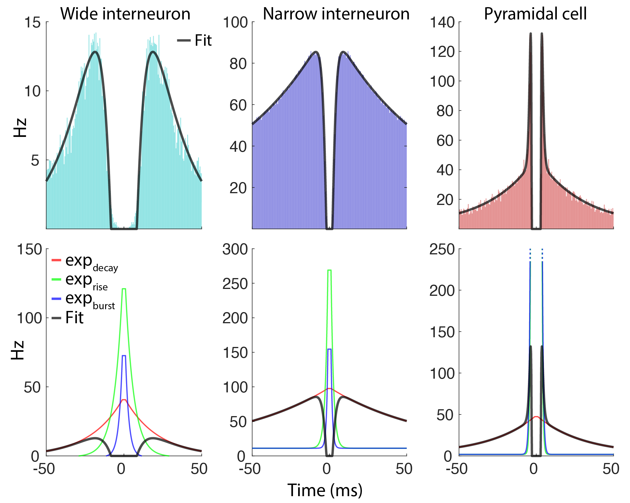
Components of the fit and example fits
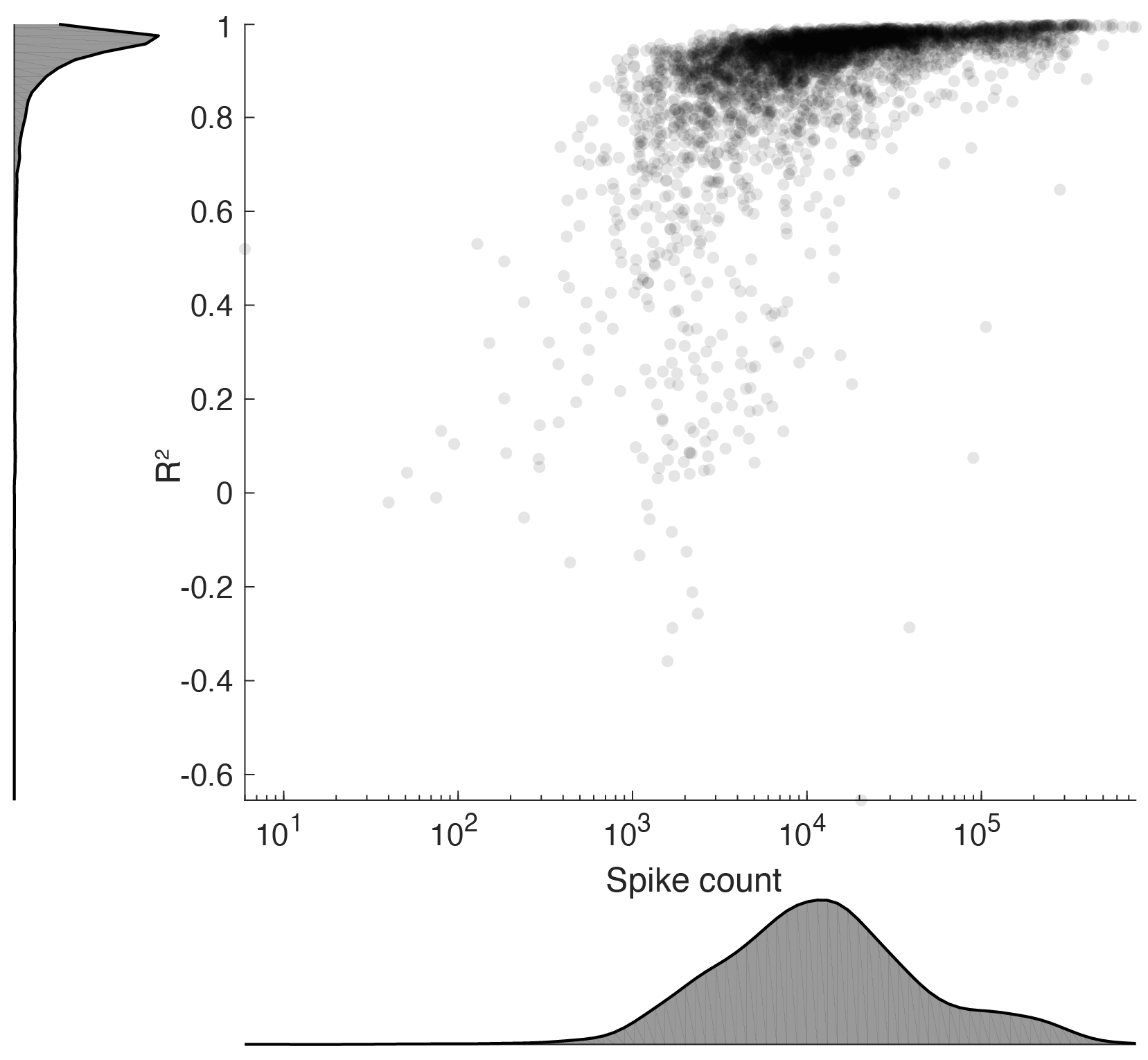
Performance
The performance is captured in below figure showing the R^2 values for each fit across 4000 hippocampal cells plotted against the number of spikes.
Limitations to the fit
The fit performs quite well for in vivo data from various brain regions, yet there are cases where this does not hold up. Manipulations should generally be excluded if it results in drastically altered spiking dynamics. Poor fit has been observed in recordings with observed seizures and other pathological conditions as well as in slice recordings where the spiking dynamics can look quite different.