UI elements of NeuroScope2
NeuroScope2 interface elements
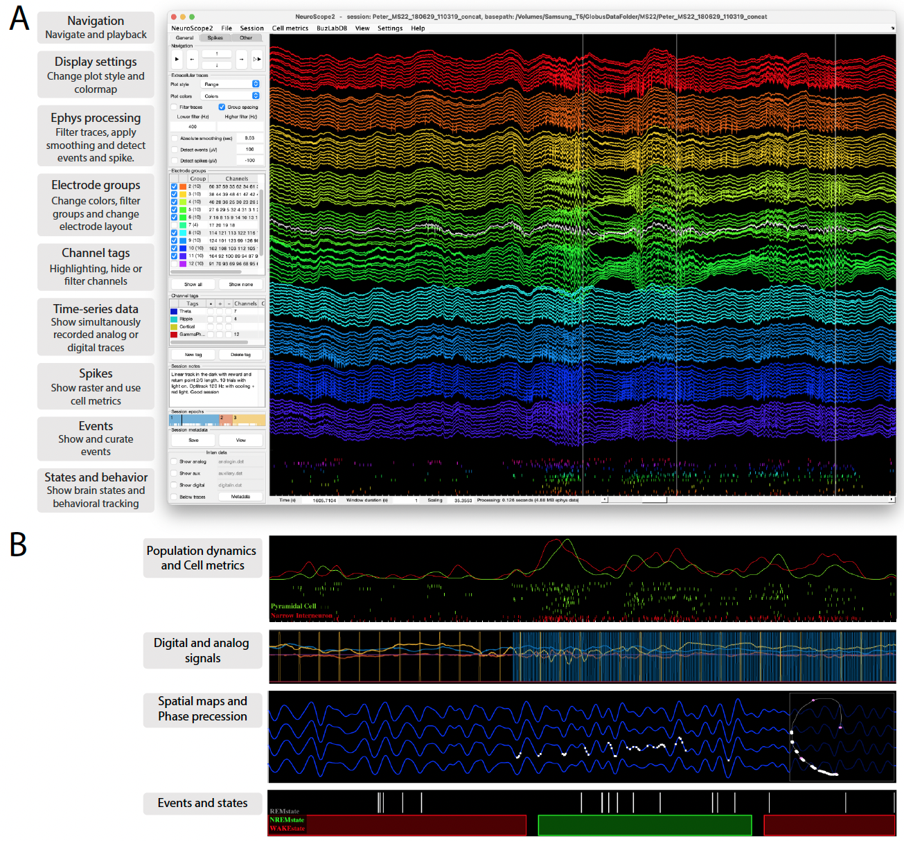
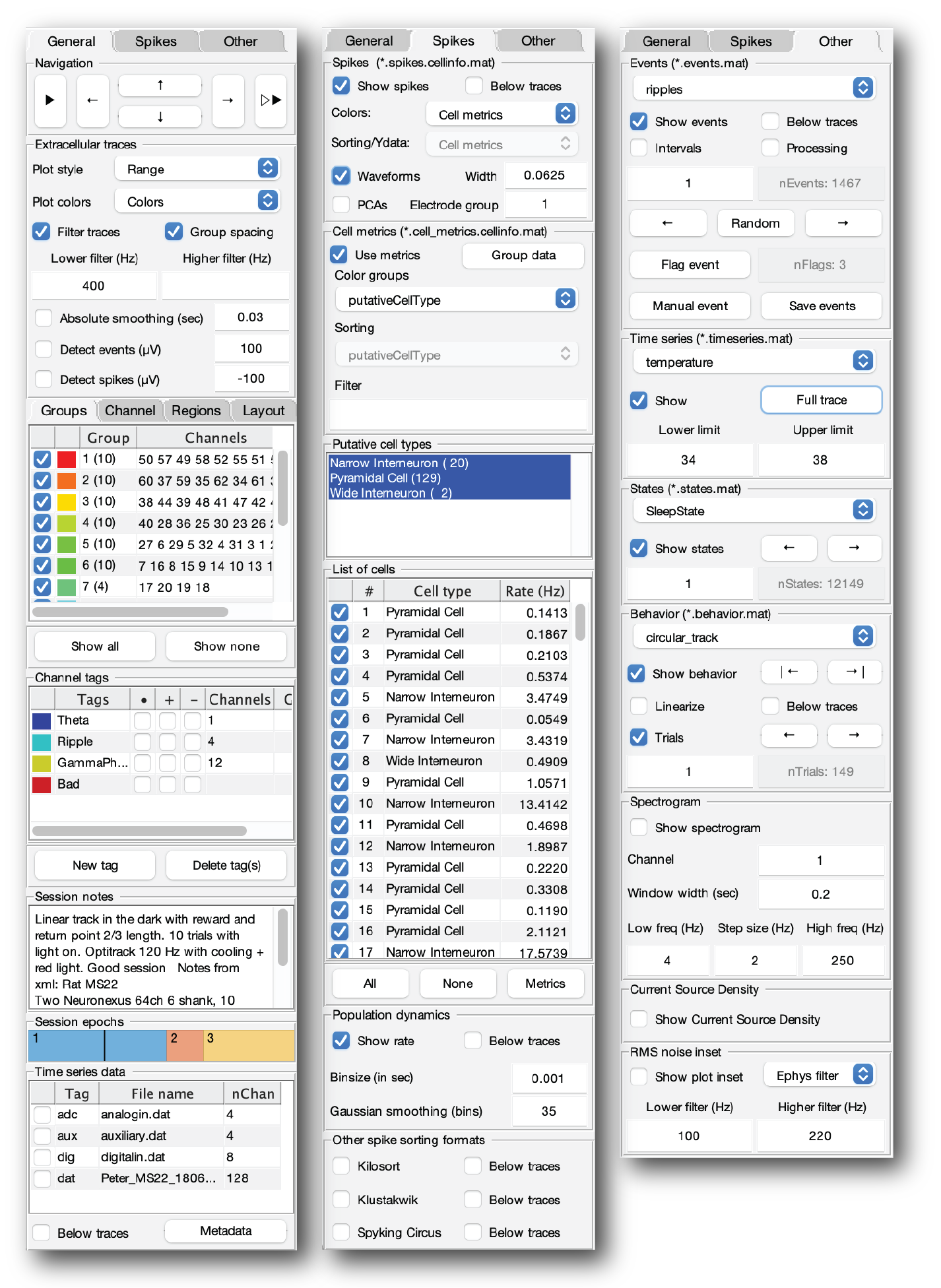
The interface consists of a side panel, a main plot axis and a navigation bar below the main axis. The side-panel has three tabs:
- General
- Navigation
- Extracellular traces
- Electrode groups
- Channel tags
- Session notes
- Session epochs
- Time series data
- Spikes
- Spikes
- Cell metrics
- Putative cell types
- List of cells
- Population dynamics
- Other spike sorting formats
- Other - other data types and data analysis, including:
- Events
- Time series
- States
- Behavior
- Spectrogram
- Current Source density visualization
- RMS noise inset
- Instantaneous metrics
- Audio playback during streaming
There are keyboard shortcuts that allow you to quickly navigate your data. Press H in NeuroScope2 to see the keyboard shortcuts.
General tab
Navigation
The Navigation panel allows you can navigate and select which cell to display.
Play icon: Stream data from current time.Left arrow: Backwards in time (quarter window length).Up arrow: Increase ephys amplitude.Down arrow: Decrease ephys amplitude.Right arrow: Forward in time (quarter window length).Double Play icon: Stream data from end of file.
Extracellular traces
Loading and plotting ephys data.
Plot style: There are six plot styles - some optimized for performance- Downsampled: Shows every 16th sample of the raw data (no filter or averaging applied).
- Range: Shows a sample count optimized for the screen resolution. For each sample the max and the min is plotted of data in the corresponding temporal range. The range plot have an extra setting allowing for a dynamic switching between
- Raw: Raw data at full sampling rate
- LFP: Shows content of a .LFP file, typically the raw data has been lowpass-filtered and downsampled to 1250Hz before this. All samples are shown.
- Image: Raw data displayed with the
imagescfunction - No ephys traces When navigating a recording, only data not currently in memory (shown on the screen) will be loaded.
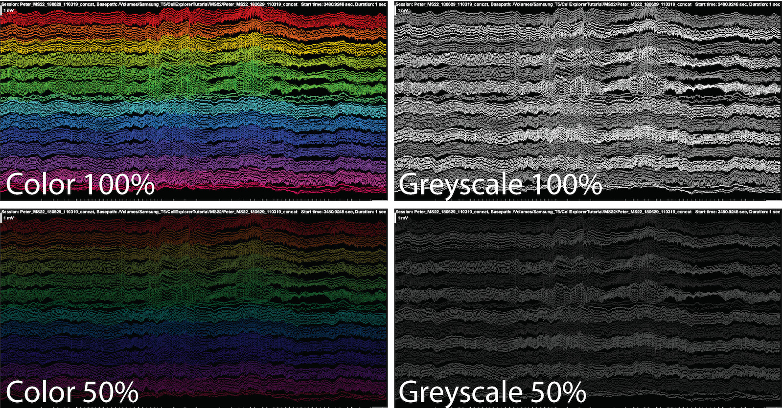
Plot color: Allows you to select from four color intensities (100%, 75%, 50%, and 25%) and four grey scale intensities (100%, 75%, 50%, and 25%) for the ephys traces. Use this when projecting spikes or events on the traces to better highlight them.
Filter traces: Apply a filter to the traces using the Lower and Higher filter setting input fields. If the Lower filter field is empty, only a low-pass filter will be applied. If the Higher filter is empty, only a high-pass filter will be applied. The filter applied is a 3rd order Zero-phase digital butter filter (filter function:filtfilt, filter design:butter).Group spacing: Adds extra spacing between traces belonging to different electrode groups.Detect events (µV): Detects events above/below the specified threshold across all channels, in units of µV (above a positive threshold; below a negative threshold).Detect spikes (µV): Detects spikes above/below the specified threshold across all channels, in units of µV (above a positive threshold; below a negative threshold). Spikes are detected on the 500Hz High-pass filtered traces (3rd order Zero-phase digital butter filter).
List of electrode groups, Channels, Regions and Layout
This panel allows for selecting channel configurations using the electrode groups, the full list of channels, brain regions assignments and electrode layout. In the list of electrode groups, groups can be selected or hidden, and the colors can be altered by clicking the colores squares. In the layout panel, channels are selected by drawing a square on top of the electrode sites. The square can be moved and boundaries altered by dragging the square. The layout tab requires the Image Processing Toolbox.
Channel tags
Channel tags allows you to highlight, filter and hide channels, using tags. The color of the highlighting can be altered by clicking the colored squares. Channel tags can be created and deleted directly from the panel.
Session notes
Allows you to see and edit session notes.
Session epochs
The session epochs panel shows a temporal axis color coded by epochs (session.epochs). The current timestamp is shown with a black line. Events are highlighted by white rasters. A left mouser click on the axis will jump to that relative time-point. Right mouse click on an epoch will jump to the beginning of that epoch. The middle mouse click allows for navigation of shown events (white raster).
Time series data
Time series are extra data which can be shown together with the primary ephys data. This includes analog and digital signals. The time series are defined i the session struct session.timeSeries and can be edited with the session GUI. Time series can be shown on top of the ephys traces (normalized range) or below the ephys traces.
Spikes tab
Spikes
Show spikes: Shows spikes data if available (basename.spikes.cellinfo.mat).Below traces: Plot spike rasters below the ephys traces.Colors: Defines the color groups (UID, Single color, Electrode groups, Cell metrics)Sorting/Ydata: Metric used for vertical sorting units when plotting them below the ephys traces.Waveforms: Show spike waveforms below traces. A spike waveform from the peak channel will be shows below the traces for each spike, arranged by the electrode layout. 1.6ms spike width by default. The Relative width of the waveforms can be adjusted.PCAs: Show PCA projection of the spike waveforms in a plot inset. This calculation will only apply for one electrode group at the time. The electrode group can be selected.
Cell metrics
Use metrics: Load cell metrics if available (basename.cell_metrics.cellinfo.mat). Cell metrics can be used for sorting, filtering and grouping cells,Group data: Allows for filtering cells by group tagsColor groups: Group cells by a cell metric (e.g. putative cell type, monosynaptic effect, brain regions or other labels)Sorting: Cell metric used for vertical sorting units when plotting them below the ephys traces.Filter: Text filter applied to character fields in cell metrics to filter cells by.
Putative cell types
Filter cells by putative cell type labels.
List of cells
List of cells allowing for selection of cells.
Population dynamics
Shows the population average spiking rate.
Below traces: Show the firing rate curves below the ephys tracesBinsize in sec: Bins/Step size of the firing rate calculations. Default: 1ms.Gaussian smoothing (bins): Width of a Gaussian smoothing kernel (in bins; ~ 2 standard deviations; default 35 bins). No kernel is applied if set to zero.
Other spike sorting formats
Allows for plotting single units from KiloSort, KlustaKwik or Spyking Circus data files.
Other tab
Events
Events files (basename.eventName.events.mat) are automatically detected and listed in the top drop-down field. Select from the list to load it. Events can be navigated either through event numbers, randomly or by using the left and right arrow buttons.
Show events: Show events as vertical lines.Below traces: Show events below the ephys traces.Intervals: Show intervals for each event if the data is available.Processing: Show extra field data available from subfields in the events struct:eventName.processing_steps.*Save events: Save any changes to the applied events file.Event number text field: Navigate to specific event. Shows the current active event.Random: Navigate to a random event.Flag event: Flag selected event. Flagged events are saved to the events structeventName.flaggedby their index id. Make sure to save the events before closing CellExplorer.+ event: Create an event manually by clicking the traces. Added events are saved to the events structeventName.addedby the timestamps. Manually added events are color coded magenta. Events can be deleted again by right clicking the events on the plot+ interval: Create intervals manually by clicking the traces. Added intervals are saved to the events structeventName.added_intervals. Manually added intervals are color coded blue. The boundaries of the intervals are defined by left mouse clicks, complete with right mouse click, cancel last point with middle mouse click. Intervals to color coded blue.- interval: Remove intervals manually by clicking the traces. Removed intervals are only affecting the manually selected intervals, which are saved toeventName.added_intervals. The boundaries of the intervals to remove are defined by left mouse clicks, complete with right mouse click, cancel last point with middle mouse click. Intervals to delete er color coded red.
Make sure to save events before closing CellExplorer if changes has been made.
Time series
Time series files (basename.timeseriesName.timeseries.mat) are automatically detected and listed in the drop-down field. Select from the list to load it.
Show: Show selected time serie on top of the ephys traces in the range defined in the limit text fields.
States
States files (basename.statesName.states.mat) are automatically detected and listed in the drop-down field. Select from the list to load it. States can be navigated either through state numbers or by using the left and right arrow buttons.
Behavior
Behavior files (basename.behaviorName.behavior.mat) are automatically detected and listed in the drop-down field. Select from the list to load it. Behavior data can be shown as a 2d projected plot inset, or as a linearized version on the main plot axis.
Behavioral trials (basename.behaviorName.behavior.mat) can be navigated either through trial number or by using the left and right arrow buttons.
Spectrogram
Shows a spectrogram below the ephys traces from specified channel. The window width (in seconds) can be altered, together with the frequency span and frequency step size (Hz).
Current Source Density
Shows a Current Source Density (CSD) on top of the ephys traces.
RMS noise inset
Shows a RMS noise inset for all channel in the upper right corner. The raw traces, the current filters or a custom filter can be used. The custom filter is specified by the lower and higher filter settings (Hz). The filter applied is a 3rd order Zero-phase digital butter filter.
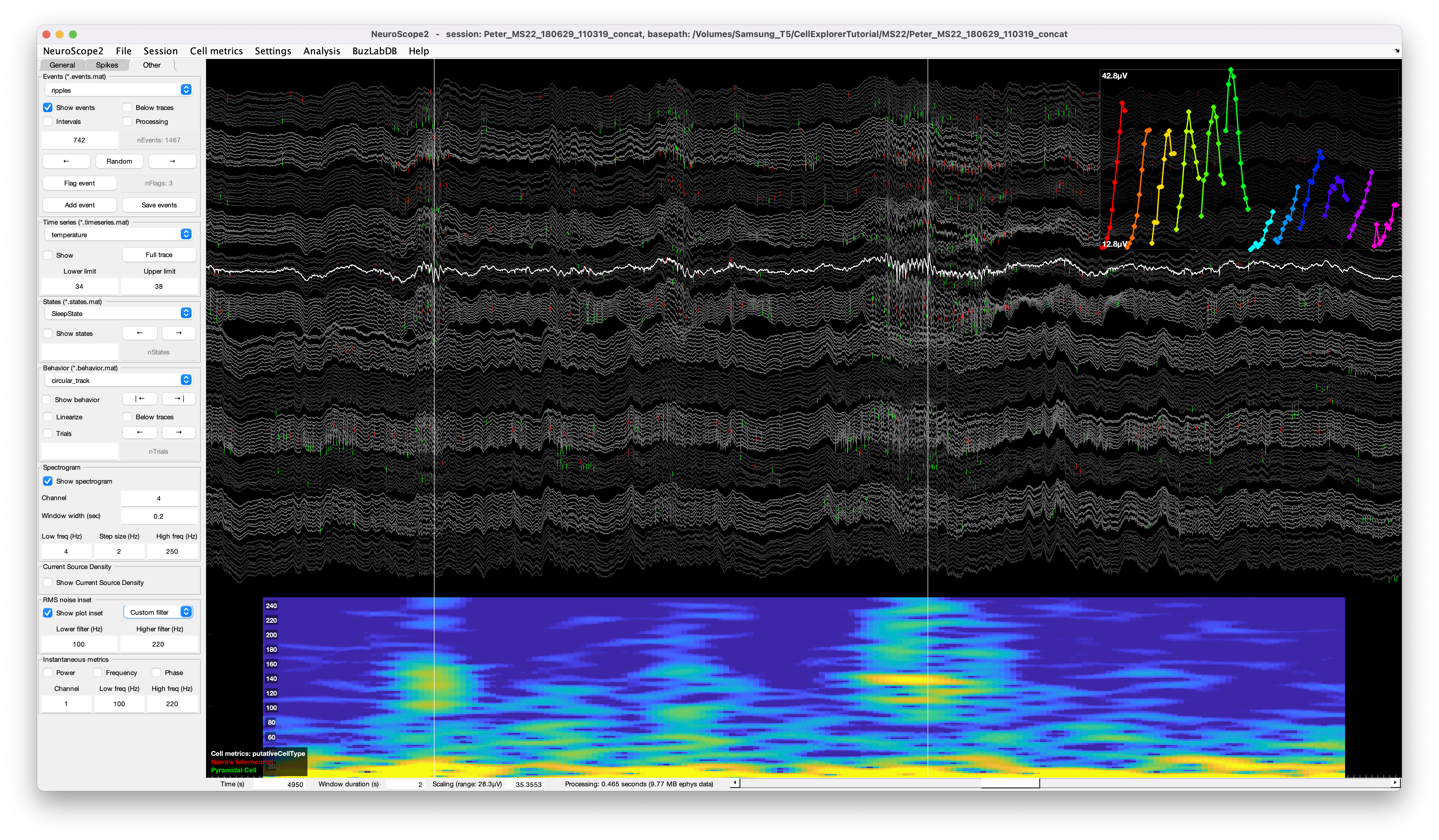
The screenshot above shows a 128 channels recording with a spectrogram shown below the traces for the channel highlighted in white. A RMS-noise channel-inset is shown in the upper right corner, showing the signal RMS-amplitude across the color-coded channels, The RMS-amplitude was calculated from the filtered traces (custom filter: 100Hz to 220Hz) . The spike raster is color-coded and sorted by putative cell types.
Instantaneous metrics
Shows the instantaneous power, phase, frequency and filtered trace from a single channel with custom filters. The channel and filter boundaries can be adjusted. The instantaneous traces are shown below the ephys traces. The filter is a third-order butter filter applied in both directions (filtfilt). The phase and power is calcuated from the hilbert transform. The frequency is calculated from the unwrapped phase: frequency = diff(unwrap(phase))./diff(timestamps)/(2*pi).
Audio playback during streaming
The traces of a one or two channels can be played as a continues audio trace as you are streaming a recording. You can select gain and specific channels to listen to (one or two channels). The audio playback is done after the filters are applied.