Channel maps tutorial
This tutorial will show you how to generate and use the two channel maps available in CellExplorer: 1. Channel coordinates (2D probe layout) and 2. the Common Coordinate Framework (CCF; by the Allen Institute). The data formats are defined here. The channel maps are useful to see the spatial location of the cells, in 2D or in 3D.
Table of contents
Channel maps examples in CellExplorer
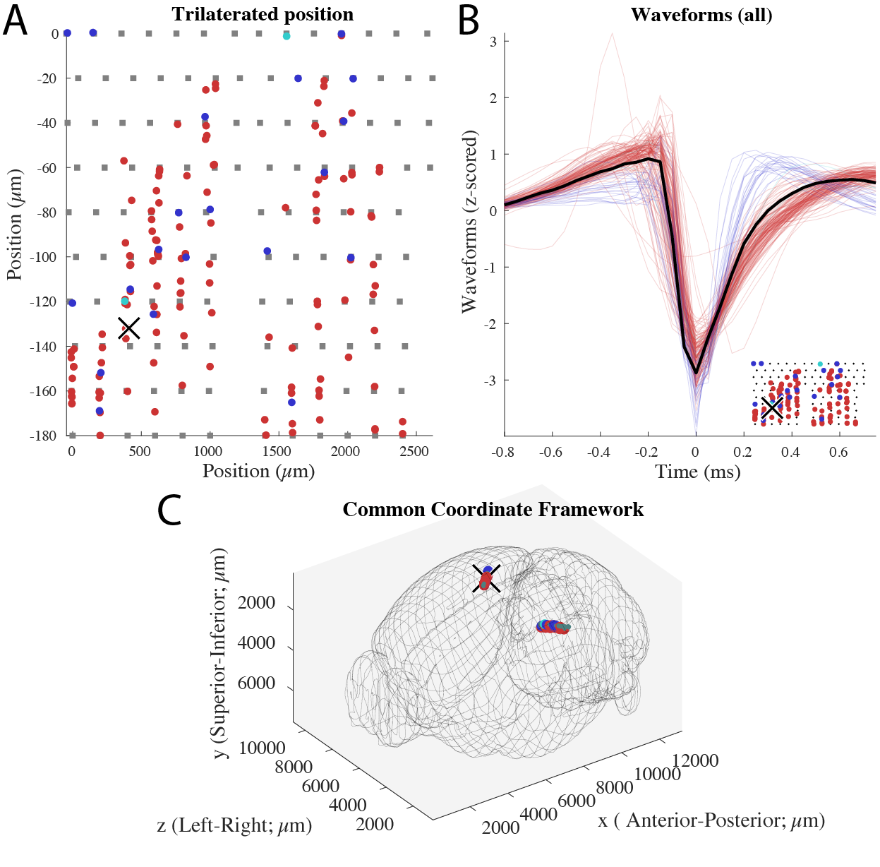
CellExplorer can show both channel maps as separate plots as shown in below figure. The probe layout can also be shows as an embedded plot in the waveform plots. The same session and cell are shown in all three panels. Two Buzsaki probes with 6 shanks (10 staggered channels per shank), implanted in CA1 in both hemispheres.
Channel coordinates (Probe layout)
The channel maps can be generated manually or with two CellExplorer functions. When you generate the channel maps manually, make sure to save them according to the data structure of CellExplorer.
Manually generating the channel coordinates
The channel coordinates are based on x and y coordinates in µm. To generate a channel map for a linear probe with 16 channels spaced 20 µm apart, you can do the following:
chanCoords.x = zeros(16,1); % Setting x-position to zero
chanCoords.y = -20*[0:15]'; % Assigning negative depth values, starting at y=0 for channel 1
That’s it! Now save that struct to the basepath as a channelInfo.mat container:
saveStruct(chanCoords,'channelInfo','session',session);
This will save the channel coordinates to a .mat file in the basepath, using the session struct to determine the basepath and basename, e.g. basepath/basename.chanCoords.channelInfo.mat. The processing pipeline will automatically detect the file and determine the position of the cells relative to the layout.
Generating the channel coordinates from session parameters
Channel coordinates can be generated from a session struct with defined electrode groups, and a couple of extra parameters: between the sites. There are two ways to provide these parameters
1. Using animal probe implants metadata
Open the session gui:
session = session_gui(session);
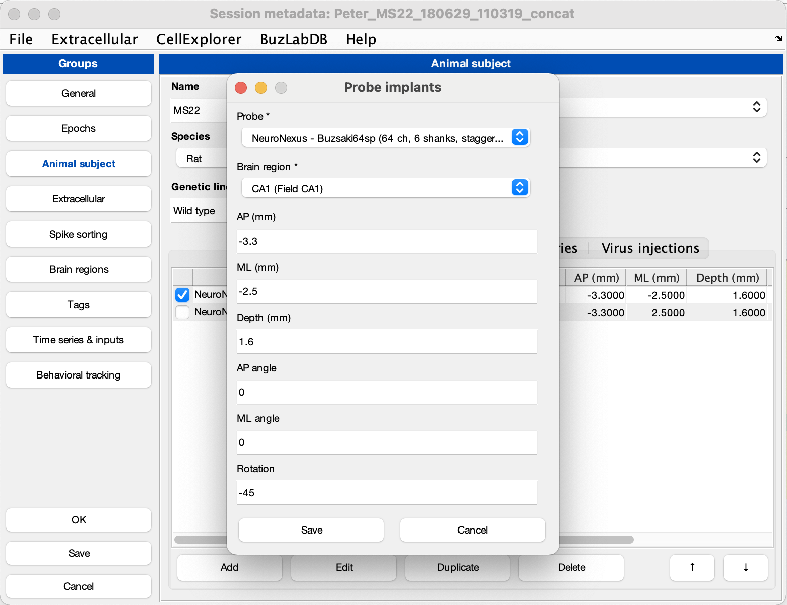
Select the Animal Subject tab in the left side-menu. Activate the Probe implants tab and click Add. This will open a probe implants window allowing you to provide probe implants information, including your probe, brain region and implant coordinates (see screenshot below). Now, to generate the channel map, close the session gui and run the script below.
generateChannelMap(session)
2. Using analysis tags
The other option is providing basic parameters about your probe geometry:
- Probe layout:
session.analysisTags.probesLayout. Select from the following options:linear: one column of channels sitting along the same linear axis (e.g. A1x16-3mm-25-177 from NeuroNexus).poly2: channels sitting in two columns, in a triangular fashion (default option; e.g. A1x16-Poly2-5mm-50s-177 from NeuroNexus).poly3: three columns of channels (e.g. A1x32-Poly3-5mm-25s-177 from NeuroNexus).poly4: four columns of channels (e.g. A2x32-Poly5-10mm-20s-200-100 from NeuroNexus).poly5: 5 columns of channels.staggered: channels are staggered with a constant vertical spacing, but an increased horizontal spacing. Channels are typically placed along the outer edge of the probe (e.g. the Buzsaki64-H64LP from NeuroNexus).
- Vertical spacing:
session.analysisTags.probesVerticalSpacing(default= 20 µm). The vertical spacing between neighboring channels. - The inter-shank distance: 200 µm (not adjustable).
% A session struct with electrode groups:
session.extracellular.electrodeGroups

% And probe layout:

generateChannelMap(session)
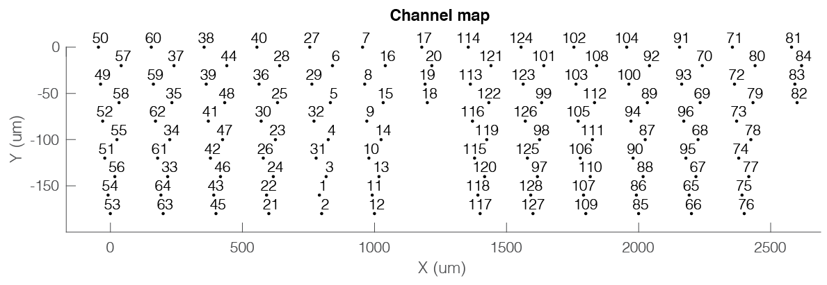
The channel map can also be generated directly from the session gui, by selecting Generate channel map from the Extracellular menu. This will generate the chanCoords file and below figure showing an example layout with two NeuroNexus Buzsaki 64 channel probes with a staggered configuration with 8 shanks (200 µm apart).
3. Generating and using channel coordinates for probe design
CellExplorer also supports true probe geometries, which must be saved as a chanCoords struct in the CellExporer directory: +chanCoords/probe_name.probes.chanCoords.channelInfo.mat. If a probe design has been defined, CellExplorer prioritizes this above other methods.
Prioritized order for generating the chanCoords file:
- Probe design
- Animal probe implants metadata
- Analysis tags
Common coordinates (CCF)
The common coordinate framework has been developed for mice, but is usable for other rodents as well, yet you will have to scale your coordinates to the mouse brain if you are using another rodent.
1. Generate common coordinates manually
The common coordinates are based on x, y and z coordinates in µm. To generate a channel map for a linear probe with 16 channels spaced 20 µm apart, you can do the following:
ccf.x = zeros(16,1); % Setting x-position to zero
ccf.y = zeros(16,1); % Setting y-position to zero
ccf.z = -20*[0:15]'; % Assigning negative depth values, starting at y=0 for channel 1
That’s it! Now, save that struct to the basepath as a channelInfo.mat container file:
saveStruct(ccf,'channelInfo','session',session);
2. Translating the probe layout to CCF coordinates
Following the one of the first two solutions for generating the channel coordinates, you can now also generate the projected CCF coordinates:
generateCommonCoordinates(session)
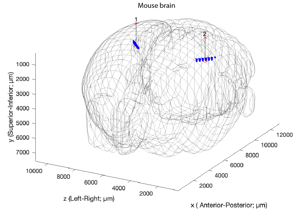
This action requires the implant metadata, and will generate a ccf file, e.g. basepath/basename.ccf.channelInfo.mat and show the figure below
The common coordinates can also be generated directly from the session gui, by selecting Generate common coordinates from the Extracellular menu. This will generate the chanCoords file and below figure showing an example layout with two Buzsaki 64 probes with a staggered configuration with 8 shanks (200 µm apart) implanted in CA1 in both hemispheres. The vectors signifies implant vectors, and the probes has been rotated along the implant axis to follow the curvature of the Longitudinal Axis of the Hippocampus.